Beat the Streak: Day Nine
In this blog post, I want to talk about why getting 80% success rate in beat the streak is so challenging. I believe I identified a mathematical reason for this, which I am going to share in this blog post.
First, lets look at some simple statistics that hint that 80% success should not be out of reach. In the table below, we are showing the percentage of games with a hit for the most successful batters in 2011-2019.
| batter | % Games with Hit | |
|---|---|---|
| 2011 | Jacoby Ellsbury | 0.821656 |
| 2012 | Derek Jeter | 0.812121 |
| 2013 | Michael Cuddyer | 0.807692 |
| 2014 | Jose Altuve | 0.803797 |
| 2015 | Dee Gordon | 0.800000 |
| 2016 | Mookie Betts | 0.807453 |
| 2017 | Ender Inciarte | 0.775641 |
| 2018 | Jose Altuve | 0.786207 |
| 2019 | DJ LeMahieu | 0.798701 |
From this table, we see that individual batters often achieved at or near 80% success rate, and therefore it's reasonable to expect that as contestants of beat the streak, we can identify more favorable situations where the probability is even higher than this by looking at matchup factors and other context. Unfortunately, I believe these empirical probabilities are misleading, and are actually a result of sampling error and hindsight bias.
Problem Abstraction
Suppose we have a collection of batters $ i=1, \dots, 250$, and each batter has a certain (unknown) probability of getting a hit in a given game $p_i$. Moreover, assume each batter plays in $162$ games, and that the outcomes for each player across games is i.i.d. For the purposes of this problem abstraction, let's assume $p_i \sim Beta(68, 32)$. This distribution is illustrated in the figure below:
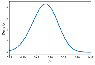
We can see from this plot that the average value of $p_i$ is $0.68$, and it can deviate roughly by $ \pm 0.12$ on either side. Now we don't observe $p_i$ directly, but we do observe the outcome all $162$ games, which is a sample from a binomial distribution with parameter $p_i$. Specifically, we have $ n_i \sim Binomial(162, p_i) $ and the empirical success rate, which we also observe, is $ \hat{p}_i = \frac{n_i}{162} $. We know that $\hat{p}_i$ is an unbiased estimator for $p_i$, so it stands to reason that it would be a reasonable approximation of it. Let's check that empirically by comparing $\hat{p_i}$ to $p_i$ and see what the resulting plot looks like.

In this experiment, the best true probability was $81.1\%$, and the highest empirical frequency was $83.3\%$. However, the player with the highest empirical frequency only had a true probability of $77.9\%$. We can thus clearly see that we have been misled by the empirical frequencies here. These results are not an artifact of one particular trial with unlucky randomness. If we repeat the experiment multiple times, the best empirical frequency was $3.5\%$ better than the best true probability on average. Furthermore, the difference between the best empirical frequency and the corresponding true probability of that (suboptimal) player, there is a massive $6\%$ difference on average.
I think this example cleanly explains why achieving 80% success rate in beat the streak is so hard, even though there are individual players who do achieve that. The problem is, we do not know which players will achieve that rate before the season starts, we can only look at the statistics in hindsight at the end of the season. Indeed, as we can see from the table above, the most successful batter changed year-to-year, with Jose Altuve being the only player to appear twice. To make matters worse, when we are making decisions about which player to pick, we will not have access to $162$ games worth of information, unless we want to draw on data from prior years. This introduces even more variance, and can magnify the effect we saw earlier.
Comments
Post a Comment