Interpolation Search Explained
If you have taken an introductory computer science course, you've probably seen the binary search algorithm - an algorithm to efficiently find the index of an item in a sorted array, if it exists. You might not have heard of interpolation search, however. Interpolation search is an alternative to binary search that utilizes information about the underlying distribution of data to be searched. By using this additional information, interpolation search can be as fast as $O(log(log(n)))$, where $n$ is the size of the array. In this post I am going to talk about two implementations of interpolation search. First, I will discuss the algorithm as described on Wikepedia, then I will describe my own version of the algorithm that has a better worst case time complexity than the first and performs better in practice than the traditional binary search and interpolation search algorithms.
Suppose for simplicity that we have a sorted array of $1000$ integers coming from a uniform distribution of integers in the range $[0,10000)$, and we wanted to find the number $2015$. Based on this information, you'd expect to find $2015$ around index $201$ or $202$ because $ \frac{2015 \cdot 1000}{10000} = 201.5 $.
There are two situations where it is possible that the key we are searching for is outside of the range determined.
Using the example from the previous two sections, this algorithm would establish a range of $[163,240]$, which will contain the key approximately $99.7\%$ of the time. The range can be increased to improve this probability. Let me explain how this range is determined.
Let $m$ be the index of the key, or if it doesn't exist, the index where it should be. Then clearly the maximum likelihood estimate for $m$ is just $201$ as determined from the previous section. Let's form a probability distribution for various values $m$ and construct a confidence interval for the index of the key. If the true index of $2015$ is $m$, then there are $m$ values in the array that are less than $2015$ and $1000−m$ values that are greater than or equal to $2015$. The probability of a random number from this distribution being less than $2015$ is $\frac{2015}{10000} \approx 0.2015$. Thus, $m$ follows a $Binom(1000,0.2015)$ distribution, so
$$ P(m)=\binom{1000}{m} \cdot 0.2015^m \cdot (1−0.2015)^{1000−m} $$
Using the normal approximation to the binomial distribution, we can say that $m$ approximately follows a normal distribution with
$$ \bar{X}=0.2015 \cdot 1000 = 201.5 \\
\sigma = \sqrt{0.2015 \cdot (1−0.2015) \cdot 1000} = 12.6 $$
Using the $68−95−99.768−95−99.7$ rule, we know that the true value of $m$ lies within $3$ standard deviations from the mean $99.7\%$ of the time,
$$ P(m \in [201.5-3 \cdot 12.6, 201.5+3 \cdot 12.6]) = P(m \in [163.4, 239.6]) = 0.997 $$
This implies that the size of the range is proportional to $ \sqrt{n} $, so the problem reduces to searching an array of size $ O(\sqrt{n}) $. We can do that in logarithmic time using binary search, so the overall time complexity of this algorithm is $ O(log(\sqrt{n})) $ with probability $ 0.997 $, and $ O(log(n)) $ with probability $0.003$. However,
$$ O(log(\sqrt{n})) = O(log(n^{1/2})) = O(\frac{1}{2} log(n)) = O(log(n)) $$
so it has the same asymptotic time complexity as binary search but has a smaller constant in front. While this is not asymptotically as fast as the first implementation, it can be applied in a wider variety of situations and the worst case time is better. An additional step you could take is to dynamically figure how big of a range you want to narrow it down to based on the size of the array and the cost of a lookup, instead of using a range of $ 3 \sigma $ no matter what.
The nice thing about this approach is that the underlying distribution does not need to be uniform. For instance, we could easily modify this search to look for names in a database. The central limit theorem allows us to use normal approximation no matter what the initial distribution is, assuming the array is large enough. Since we are interested in performance for very large array sizes, we can make this assumption. The distribution of the first letter in English names is not uniform, but as long as you know the probability that a random name is less than the name your searching for, you can apply this analysis all the same. The ability to easily generalize this approach makes it a great candidate for improving search performance. You can find this information online, or do a one-pass though your list of names and calculate the distribution yourself.
A test consists of building a sorted array of $n$ integers in the range $[0,n)$ and searching for all the numbers that could possibly be in the distribution one by one. While this is not the most efficient way to answer this question, it serves it purpose to benchmark the different algorithms. Here are the results:
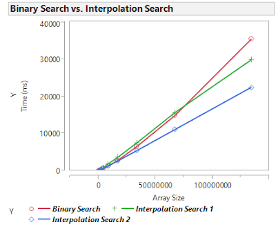
Both interpolation searches perform better for sufficiently large $n$ than the binary search, but it takes the first implementation longer to overcome the binary search. Even though the first implementation has smaller theoretical time complexity, the second implementation appears to perform better up to and beyond $n=2^{27}$.
The Basic Idea
Interpolation search models how humans search a dictionary better than a binary search, because if a human were to search for "Yellow", they would immediately flip towards the end of the dictionary to find that word, as opposed to flipping to the middle. This is the fundamental idea of how interpolation search works.Suppose for simplicity that we have a sorted array of $1000$ integers coming from a uniform distribution of integers in the range $[0,10000)$, and we wanted to find the number $2015$. Based on this information, you'd expect to find $2015$ around index $201$ or $202$ because $ \frac{2015 \cdot 1000}{10000} = 201.5 $.
Implementation 1
Assume we are searching from a uniform distribution as described in the previous section, and the first index we check is $201$. If the actual value at that index is $2250$, then we recursively reduce the problem by searching the left sub-array. We must also refine the distribution to a uniform distribution with integers in the range $[0,2250]$. The next index we check is $ \frac{2015 \cdot 201}{2250} \approx 180$. If the value at that index is $2010$, then we search the right sub-array with the new distribution $[2010,2250]$. The next index we search is $180+\frac{(201−180)(2250−2010)}{2015} \approx 183$. We repeat this process until we've found the item we're searching for or we've narrowed down he search space to $0$ elements. There are two main drawbacks of this approach:- If the underlying distribution is not uniform, then the time complexity can be as bad as $O(n)$.
- If the underlying distribution is not uniform, it's difficult to implement this algorithm (although the mathematical theory still works out).
Implementation 2
This implementation addresses the two drawbacks of the previous implementation by ensuring $O(log(n))$ performance regardless of the initial distribution. Instead of trying to pinpoint the exact index that the key we are searching is in, we establish a range that will contain the value with high probability. Once that range is established, the traditional binary search algorithm is used on the reduced problem.There are two situations where it is possible that the key we are searching for is outside of the range determined.
- The distribution is not what we originally assumed.
- The distribution is what we originally assumed, but there is still a small probability that the key lies outside the range.
Using the example from the previous two sections, this algorithm would establish a range of $[163,240]$, which will contain the key approximately $99.7\%$ of the time. The range can be increased to improve this probability. Let me explain how this range is determined.
Let $m$ be the index of the key, or if it doesn't exist, the index where it should be. Then clearly the maximum likelihood estimate for $m$ is just $201$ as determined from the previous section. Let's form a probability distribution for various values $m$ and construct a confidence interval for the index of the key. If the true index of $2015$ is $m$, then there are $m$ values in the array that are less than $2015$ and $1000−m$ values that are greater than or equal to $2015$. The probability of a random number from this distribution being less than $2015$ is $\frac{2015}{10000} \approx 0.2015$. Thus, $m$ follows a $Binom(1000,0.2015)$ distribution, so
$$ P(m)=\binom{1000}{m} \cdot 0.2015^m \cdot (1−0.2015)^{1000−m} $$
Using the normal approximation to the binomial distribution, we can say that $m$ approximately follows a normal distribution with
$$ \bar{X}=0.2015 \cdot 1000 = 201.5 \\
\sigma = \sqrt{0.2015 \cdot (1−0.2015) \cdot 1000} = 12.6 $$
Using the $68−95−99.768−95−99.7$ rule, we know that the true value of $m$ lies within $3$ standard deviations from the mean $99.7\%$ of the time,
$$ P(m \in [201.5-3 \cdot 12.6, 201.5+3 \cdot 12.6]) = P(m \in [163.4, 239.6]) = 0.997 $$
This implies that the size of the range is proportional to $ \sqrt{n} $, so the problem reduces to searching an array of size $ O(\sqrt{n}) $. We can do that in logarithmic time using binary search, so the overall time complexity of this algorithm is $ O(log(\sqrt{n})) $ with probability $ 0.997 $, and $ O(log(n)) $ with probability $0.003$. However,
$$ O(log(\sqrt{n})) = O(log(n^{1/2})) = O(\frac{1}{2} log(n)) = O(log(n)) $$
so it has the same asymptotic time complexity as binary search but has a smaller constant in front. While this is not asymptotically as fast as the first implementation, it can be applied in a wider variety of situations and the worst case time is better. An additional step you could take is to dynamically figure how big of a range you want to narrow it down to based on the size of the array and the cost of a lookup, instead of using a range of $ 3 \sigma $ no matter what.
The nice thing about this approach is that the underlying distribution does not need to be uniform. For instance, we could easily modify this search to look for names in a database. The central limit theorem allows us to use normal approximation no matter what the initial distribution is, assuming the array is large enough. Since we are interested in performance for very large array sizes, we can make this assumption. The distribution of the first letter in English names is not uniform, but as long as you know the probability that a random name is less than the name your searching for, you can apply this analysis all the same. The ability to easily generalize this approach makes it a great candidate for improving search performance. You can find this information online, or do a one-pass though your list of names and calculate the distribution yourself.
Results
To explore the theoretical results in a practical environment, I implemented all three of these algorithms in Java and ran some benchmarking tests. For testing purposes, I used an implementation where for an array of size $n$, the values in the array come from a uniform distribution of integers in the range $[0,n)$. However, changing the distribution can change the results of the analysis. If the distribution is more dense, like $[0,n/2]$, then the interpolation searches become better compared to the standard binary search, but for a distribution such as $[0,10n]$, it takes longer for the interpolation searches to overcome the binary search.A test consists of building a sorted array of $n$ integers in the range $[0,n)$ and searching for all the numbers that could possibly be in the distribution one by one. While this is not the most efficient way to answer this question, it serves it purpose to benchmark the different algorithms. Here are the results:

Both interpolation searches perform better for sufficiently large $n$ than the binary search, but it takes the first implementation longer to overcome the binary search. Even though the first implementation has smaller theoretical time complexity, the second implementation appears to perform better up to and beyond $n=2^{27}$.
Conclusion
Binary search is already so blazingly fast, that you probably don't have much need to use an interpolation search, unless you are searching through billions of entries worth data, or the cost of a lookup is expensive so minimizing the number of lookups is crucial. However, interpolation search is an interesting algorithm nonetheless, and can be the right choice in some cases. Summing up the results, there are a number of things you should keep in mind when implementing a search algorithm:- The second implementation has the same theoretical performance as binary search, but it outperforms binary search in practice.
- The second implementation outperforms the first interpolation search for pretty large array sizes.
- The second implementation can easily be generalized for searching through other distributions, such as usernames in a database.
- The first implementation has the best theoretical performance, but it takes a while to overcome binary search and the second implementation of interpolation search.
- Both versions of interpolation search work well when the cost of an array lookup is much greater than the index computations on the CPU.
Comments
Post a Comment