Generating Random Numbers from Arbitrary Distributions
Generating random numbers is an important aspect of programming, and just about every programming language offers some source of (pseudo) randomness, usually in the form of a uniform distribution. For example, java has a builtin function, <code class="java">Math.random()</code> that returns a random floating point number in the range $[0,1)$. In some instances, we would like to have random numbers coming from a different distribution, but most programming languages don't offer this functionality (except very specialized languages such as R). In the rest of this blog post, I am going to explain how you can use a uniformly distributed random number to generate a number from some other distribution.
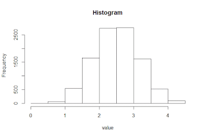 Looks approximately normal, right? Not bad - that was pretty easy.
 This method works nicely and is pretty simple to implement given that you have a suitable range of acceptable values, but it is non-deterministic and therefor not an ideal solution.
 As you can probably see, the random die roll is the smallest value of $K$ such that $P(X \leq K)$ is greater than $r$, where $r$ is the uniform random number supplied by the system. This applies to the discrete case, but in the continuous case it is even easier to find! Consider the CDF for the exponential distribution used in the monte carlo example.
 Let $ F(K) = P(X \leq K) $ where $X$ is an exponential random variable. If we were to apply the same reasoning to this exponential CDF, then we could use our uniform random number to calculate $X$ by solving the equation $F(X)=r$, where again $r$ denotes the uniform random number from $[0,1)$ that is supplied from the system. This is just the continuous analogy of the discrete case I described earlier.
Solving the equation $F(X)=r$ can be somewhat tricky, and depending on the situation you may have to appeal to different methods. In general, the CDF can be computed as the integral of the PDF. Once the CDF is calculated, the function must be inverted. It is possible that either of these steps cannot be done algebraically and thus you must use computational methods instead. If you are unable to find the indefinite integral of the PDF, you can use a numerical integration technique such as the trapezoidal rule or Simpson's rule to numerically evaluate the CDF. If you can find the CDF but it's not invertable, then you will need to use some other method to find the value of XX corresponding with the equation $F(X)=r$. Since the CDF is non-descending (this is a direct result of the definition), you can think of it as a sorted list of numbers and apply a divide and conquer binary search type solution to zero in on the value of $X$ such that $F(X)=r$.
Depending on which of the three situations you find yourself, you may have different performance from these solutions. If you can invert the CDF, then it's easy and you can perform the transform in $O(1)$. If you can find the indefinite integral of the PDF (and get the CDF), then you can perform the transformation in $O(\log{n})$ where $n$ is a function of the desired accuracy, and can be tuned to trade some digits of precision for efficiency. If you have to numerically evaluate the integral to compute the CDF, then the performance depends on your implementation, but it is going be the slowest of the three solutions so you should try to avoid this situation if at all possible.
Special Case: The Normal Distribution
If you would like to get numbers from a binomial distribution, or are willing to accept an approximation for the normal distribution in favor of simplicity, then you may want to use this technique. If you add together some number (n) of uniform random variables, the distribution is binomial; as you increase n, this distribution approaches the normal distribution and it converges pretty quickly. This is called the Central Limit Theorem, and it applies to any distribution, not just the uniform (the sum of random variables from any distribution converges to the normal distribution in the limit). For example, by summing 5 uniform random variables 10000 times, we get the following histogram.
Monte Carlo Approach
In general, the approach described above does not work; it only applies to the normal distribution. If we wanted to generate random variables from some other distribution, then we would need to appeal to a different technique. One such approach is to run a Monte Carlo simulation. This approach is not the main approach that I would like to outline in this post, so I will not spend too much on but here is the basic idea. Repeatedly generate two random numbers in a suitable domain, if the point given by the two random numbers lies under the distribution function, then accept the x value as the random number. Otherwise, repeat the process by picking two new random numbers. For example, for the exponential distribution, the process could look something like this, resulting in a value of 1.3 to be generated:
Using the Cumulative Distribution Function
In general, with a little bit of math, you can calculate the cumulative distribution function (CDF) from a probability density function (PDF) and use this information to generate a random number from this distribution. Consider the trivial example of generating a random integer from ${1,2,3,4,5,6}$ using a uniformly random number from $ r \in [0,1) $. One way to do this is by defining the following piece-wise function:def roll(r):
if(r < 1/6):
return(1)
elif(r < 2/6):
return(2)
elif(r < 3/6):
return(3)
elif(r < 4/6):
return(4)
elif(r < 5/6):
return(5)
else
return(6)
def roll(r):
  return floor(r*6)+1


Solving the equation $F(X)=r$ can be somewhat tricky, and depending on the situation you may have to appeal to different methods. In general, the CDF can be computed as the integral of the PDF. Once the CDF is calculated, the function must be inverted. It is possible that either of these steps cannot be done algebraically and thus you must use computational methods instead. If you are unable to find the indefinite integral of the PDF, you can use a numerical integration technique such as the trapezoidal rule or Simpson's rule to numerically evaluate the CDF. If you can find the CDF but it's not invertable, then you will need to use some other method to find the value of XX corresponding with the equation $F(X)=r$. Since the CDF is non-descending (this is a direct result of the definition), you can think of it as a sorted list of numbers and apply a divide and conquer binary search type solution to zero in on the value of $X$ such that $F(X)=r$.
Depending on which of the three situations you find yourself, you may have different performance from these solutions. If you can invert the CDF, then it's easy and you can perform the transform in $O(1)$. If you can find the indefinite integral of the PDF (and get the CDF), then you can perform the transformation in $O(\log{n})$ where $n$ is a function of the desired accuracy, and can be tuned to trade some digits of precision for efficiency. If you have to numerically evaluate the integral to compute the CDF, then the performance depends on your implementation, but it is going be the slowest of the three solutions so you should try to avoid this situation if at all possible.
Comments
Post a Comment