Tail Bounds on the Sum of Half Normal Random Variables
Let $ x \sim \mathcal{N}(0, \sigma^2)^n $ be a vector of $ n $ i.i.d normal random variables. We wish to provide a high probability tail bound on the $L_1$ norm of $x$, that is:
$$ Pr[|| x ||_1 \geq a] \leq f(a) $$
Note that the term on the left is called a "tail probability" because it captures the probability mass in the tail of the distribution (i.e., values exceeding a). This type of problem arises when we wish to claim that the probability is small for a given random variable to be large. The tail probability above is closely related to the CDF of the random variable $ || x ||_1 $: it is exactly $ 1 - Pr[|| x ||_1 \leq a] $. Unfortunately, the CDF of this random variable does not appear to have a clean closed form expression, and for that reason, we wish to find a reasonably clean and tight bound on it instead. In this blog post, we will explore, utilize, and compare the Markov inequality, the one-sided Chebyshev inequality, and the Chernoff bound to bound the desired tail probability.
We will begin by observing that $ || x ||_1 = \sum_{i=1}^n | x |_i $, and $ | x_i | $ is a half-normal random variable. This random variable has expectation $ \mathbb{E}[|x_i|] = \sigma \sqrt{2/\pi} $ and variance $ \mathbb{V}[|x_i|] = \sigma^2 (1 - \frac{2}{\pi}) $. By the linearity of expectation, we know:
$$ \mathbb{E}[|| x ||_1] = n \sigma \sqrt{2/\pi} $$
and since $ | x_i | $ are all independent, we know the variance of their sum is equal to the sum of their variances:
$$ \mathbb{V}[||x_1||] = n \sigma^2 (1 - \frac{2}{\pi}) $$
Markov Inequality
Markov's inequality provides a bound on the desired tail probability using only the expected value of a non-negative random variable. It says:
$$ Pr[|| x ||_1 \geq a] \leq \frac{\mathbb{E}[||x||_1]}{a} = \frac{n \sigma \sqrt{2/\pi}}{a} $$
One-sided Chebyshev inequality
Next, we will use the one-sided Chebyshev inequality, also known as Cantelli's inequality, to provide a tighter bound on the desired tail probability. This bound depends on both the expected value of the random variable, as well as it's variance. It says:
$$ \begin{aligned}
Pr[||x_1|| \geq \mathbb{E}[||x||_1] + a] &\leq \frac{\mathbb{V}[||x||_1]}{\mathbb{V}[||x||_1] + a^2} \\
Pr[||x_1|| \geq n \sigma \sqrt{2 / \pi} + a] &= \frac{n \sigma^2 (1-2/\pi)}{n \sigma^2 (1 - 2/\pi) + a^2} \\
\end{aligned} $$
Chernoff bound
Next, we will derive an even tighter bound by utilizing the moment generating function of the random variable $ || x ||_1 $. The Chernoff bound works by applying Markov's inequality to the random variable $ \exp{(t \cdot || x ||_1)}$. It says that for all $ t \geq 0$, we have:
$$ Pr[|| x ||_1 \geq a] = Pr[\exp{(t \cdot || x ||_1)} \geq \exp{(t \cdot a)}] \leq \frac{\mathbb{E}[\exp{(t \cdot || x ||_1)}]}{\exp{(t \cdot a)}} $$
In order to apply this bound, we must first derive $ \mathbb{E}[\exp{(t \cdot || x ||_1)}]$, which is known as the moment generating function of the random variable $ || x ||_1 $. It turns out that since $ || x ||_1 $ is a sum of independent random variables $ | x_i | $, the moment generating function of $||x||_1$ simplifies to the product of moment generating functions of $ |x_i| $. Moreover, since $ | x_i | $ are identically distributed, things simplify even further, and we know:
$$ \mathbb{E}[\exp{(t \cdot || x ||_1)}] = \mathbb{E}[\exp{(t | x_i |)}]^n $$
Do not let the name "moment generating function" intimidate you: we can reason about it simply by utilizing the definition of expected value, that is:
$$ \begin{aligned}
\mathbb{E}[\exp{(t | x |_i)}] &= \int_{-\infty}^{\infty} \phi(x_i/\sigma) \exp{(t \cdot | x_i |)} d x_i \\
&= 2 \int_{0}^{\infty} \phi(x_i/\sigma) \exp{(t \cdot x_i)} d x_i \\
&= \frac{1}{\sigma} \sqrt{\frac{2}{\pi}} \int_{0}^{\infty} \exp{(-x_i^2/2 \sigma^2 )} \exp{(t \cdot x_i)} d x_i \\
&= \frac{1}{\sigma} \sqrt{\frac{2}{\pi}} \int_{0}^{\infty} \exp{(-x_i^2/2 \sigma^2 + t \cdot x_i)} d x_i \\
&= \exp{(\sigma^2 t^2/2)} (1 + \Phi(t \sigma / \sqrt{2})) \\
\end{aligned} $$
Above $\phi$ and $\Phi$ are the PDF and CDF of a standard normal random variable, respectively. Note that I used WolframAlpha to simplify the last expression for me: the interested reader is free to try to work out the integral for themselves. Now plugging this expression back into the Chernoff bound, we obtain:
$$ \begin{aligned}
Pr[|| x ||_1 \geq a] &\leq \min_{t \geq 0} \frac{\mathbb{E}[\exp{(t \cdot || x ||_1)}]}{\exp{(t \cdot a)}} \\
&= \min_{t \geq 0} \frac{\exp{(\sigma^2 t^2/2)}^n (1 + \Phi(t \sigma / \sqrt{2}))^n}{\exp{(t a)}} \\
&= \min_{t \geq 0} \exp{(n \sigma^2 t^2/2 - t a + n \log{(1 + \Phi(t \sigma / \sqrt{2}))}} \\
&\leq \min_{t \geq 0} \exp{(n t^2/2 - t a + n \log{2})} \\
&\leq \exp{(n \sigma^2 (a/n \sigma^2)^2 / 2 - (a/n \sigma^2) a + n \log{2})} \\
&= \exp{\Big(-\frac{a^2}{2n \sigma^2} + n \log{2}\Big)} \\
\end{aligned} $$
Visual comparison
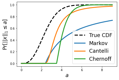
Thus far, we have derived three different bounds for the desired tail probability. However, looking at the formulas it is not exactly clear how the three bounds compare. Thus, we will now visualize the true CDF of the distribution along with the three different bounds we have derived for it. Recall that it is not obvious how to evaluate the true CDF of this distribution. Thus, we instead take 1 million random samples from the distribution and plot the empirical CDF instead. In the plot below, we use $n = 10$ and $\sigma = 1$:
Next, we will compare the bounds from a slightly different angle. In particular, we will seek to find the value of $a$ such that $ Pr[||x||_1 \geq a] \leq \delta $ (think of $\delta$ as some small value, e.g., $\delta = 0.01$).
For the Markov bound, we have:
$$ \frac{n \sigma \sqrt{2/\pi}}{a} = \delta \rightarrow a = \frac{1}{\delta} n \sigma \sqrt{2 / \pi} $$
For the Cantelli bound, we have:
$$ \frac{n \sigma^2 (1-2/\pi)}{n \sigma^2 (1 - 2/\pi) + (a - \sqrt{2 / \pi} \sigma n)^2} = \delta \rightarrow a = \sqrt{2 / \pi} \sigma n + \sigma \sqrt{(1/\delta - 1) n (1 - 2 / \pi)}$$
For the Chernoff bound, we have:
$$ \exp{\Big(-\frac{a^2}{2n \sigma^2} + n \log{2}\Big)} = \delta \rightarrow a = \sigma n \sqrt{2 \log{2}} + \sigma \sqrt{2 n \log{(1 / \delta)}} $$
While these equations seem ugly at first glance, with all the symbols, logs, and square roots, it's worth looking at them and thinking about their similarities and differences. Both the Cantelli and Chernoff bound have two terms, one which is $O(n)$ and another which is $O(\sqrt{n})$. The first term roughly corresponds to the expected magnitude of $||x||_1$ while the second term captures how much it can deviate from this expected value. On the other hand, the Markov bound has only one term that is $O(n)$ and is thus weaker than the other two in general. While the term for the Cantelli bound is smaller at first (since $\sqrt{2/ \pi}$ is less than $ \sqrt{2 \log{2}}$), the Chernoff bound has a better dependence on $\delta$ (since $ \sqrt{\log{(1/ \delta)}} \ll \sqrt{1 / \delta} $). This confirms what we saw visually above, especially for the interesting regime where $\delta$ is small.
While the Chernoff bound is the most complex of the three, it also provides the strongest bounds. In contrast, the Markov inequality is easiest to apply by provides the weakest bounds. The Cantelli bound sits in the middle: providing reasonable bounds that are simple to apply, as they only rely on knowing the expected value and variance of the random variable in consideration.
Summary
In this blog post, we applied standard inequalities from probability theory to a new problem. We showed how to bound the tail probabilities of the $L_1$ norm of a vector of i.i.d. normal random variables and compared these different bounds both visually and analytically.
Comments
Post a Comment