Solving Problems with Dynamic Programming
Dynamic Programming is a programming technique used to solve large, complex problems that have overlapping sub-problems. It does this by computing each sub-problem only once, ensuring non-exponential behavior. It differs from memoization (no, that's not a typo) in that instead of computing the result of a function then storing it in a cache, it instead generates a certain result before calculating any other result that relies on it.
Dynamic Programming problems often require a different way of thinking than typical problems. Most often, dynamic programming becomes useful when you want to reverse engineer a tree recursive function. By that I mean you want to start of with the base case(s), then use those to generate the next few cases, and repeat this process until all points of interest have been calculated. Most often, at least in imperative languages, these dynamic programming algorithms are iterative, meaning they don't have recursive calls. That being said, it's still possible to have a recursive dynamic programming algorithm, it's just not as common from what I've seen.
I will discuss a particular problem that is a good example of when and how to use dynamic programming. I programmed my solution with Java, but I will also show a few code bits from Haskell just because of how elegant it is. The problem is this:
The first thing to do is try to think up a way to count how many possibilities ensuring that you cover every case and never cover the same case more than once. This can be done with a carefully thought out recurrence relation. Let D be the denomination array and Let $C(a,b)$ be the number of ways to make change for a using only denominations less than or equal to the D[b]. Then
$$ C(a,b) =
\left\{
\begin{array}{ll}
0 & a < 0 \: or \: b < 0 \\
1 & a = 0 \: and \: b = 0\\
C(a-D[b], b) + C(a, b-1) & otherwise
\end{array}
\right. $$ The first 2 piece-wise definitions in the recurrence relation are base cases, but the true magic occurs in the general case. It is basically saying if you count the number of ways to achieve a - D[b] using denominations less than or equal to D[b], and add that to the number of ways to achieve a using denominations less than or equal to D[b-1]., you will get the number of ways to make change for a using denominations less than or equal to D[b]. I will leave it to the reader to convince yourself of it's correctness.
So how would we go about coding this? Well here is a Haskell implementation:
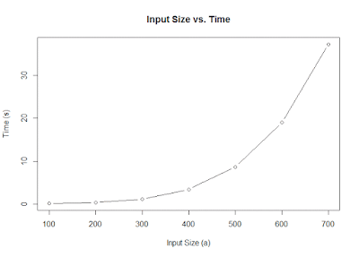
I slightly modified the above recurrence relation but the general essence is the same. The natural question to ask next is: How well does this solution scale? This implementation does not scale well because you end up doing a lot of duplicate work. For instance,
$$ C(50, 2) = C(40, 2) + C(50, 1)\\ C(40, 3) = C(35, 3) + C(40, 2) $$ As you can see both of these rely on the same result, namely $C(40,2)$. When this re-computation accumulates down the execution tree, you end up with exponential time which is never good.
$$ C(a,b) = \left\{ \begin{array}{ll} 1 & a = 0 \: and \: b = 0\\ C(a-D[b], b) + C(a, b-1) & otherwise \end{array} \right. $$ The idea behind the dynamic programming algorithm is to update related values on the fly and hope that by the time we reach any given configuration, it's been fully evaluated. If we choose our order carefully, we should be able to achieve this. Assume that we know $C(a,b)$. What does that say about other values of $C$? Well, from the recurrence relation above, exactly 2 other functions rely on this function as a partial result. Namely, $C(a+D[b],b)$ relies on the result of $C(a,b)$ and $C(a,b+1)$ also relies on the result of $C(a,b)$. Thus, whenever we get to cell $(a, b)$, we can update these 2 dependent cells.
What order should we evaluate these partial counts in? Naturally, it makes sense to start at the single known value, $C(0,0)=1$, but where should we go after that? Well, it turns out that the correct ordering is to evaluate all the denominations (in consecutive order) for low values then iteratively work your way up. Here is a Java snippet demonstrating this idea:
Dynamic Programming problems often require a different way of thinking than typical problems. Most often, dynamic programming becomes useful when you want to reverse engineer a tree recursive function. By that I mean you want to start of with the base case(s), then use those to generate the next few cases, and repeat this process until all points of interest have been calculated. Most often, at least in imperative languages, these dynamic programming algorithms are iterative, meaning they don't have recursive calls. That being said, it's still possible to have a recursive dynamic programming algorithm, it's just not as common from what I've seen.
I will discuss a particular problem that is a good example of when and how to use dynamic programming. I programmed my solution with Java, but I will also show a few code bits from Haskell just because of how elegant it is. The problem is this:
Using only the denominations $ { 50, 25, 10, 5, 1 } $, how many ways can you make change for $ 100 $?The above problem is not very large so it's easy enough to solve without dynamic programming. That being said, however, as the problem scales up (i.e., more denominations or bigger starting amount of money), dynamic programming soon becomes necessary.
The first thing to do is try to think up a way to count how many possibilities ensuring that you cover every case and never cover the same case more than once. This can be done with a carefully thought out recurrence relation. Let D be the denomination array and Let $C(a,b)$ be the number of ways to make change for a using only denominations less than or equal to the D[b]. Then
$$ C(a,b) =
\left\{
\begin{array}{ll}
0 & a < 0 \: or \: b < 0 \\
1 & a = 0 \: and \: b = 0\\
C(a-D[b], b) + C(a, b-1) & otherwise
\end{array}
\right. $$ The first 2 piece-wise definitions in the recurrence relation are base cases, but the true magic occurs in the general case. It is basically saying if you count the number of ways to achieve a - D[b] using denominations less than or equal to D[b], and add that to the number of ways to achieve a using denominations less than or equal to D[b-1]., you will get the number of ways to make change for a using denominations less than or equal to D[b]. I will leave it to the reader to convince yourself of it's correctness.
So how would we go about coding this? Well here is a Haskell implementation:
count :: Int -> [Int] -> Int
count 0 _ = 1
count _ [] = 0
count a (d:ds)
  | a < 0 = 0
  | otherwise = count (a-d) (d:ds) + count a ds
I slightly modified the above recurrence relation but the general essence is the same. The natural question to ask next is: How well does this solution scale? This implementation does not scale well because you end up doing a lot of duplicate work. For instance,
$$ C(50, 2) = C(40, 2) + C(50, 1)\\ C(40, 3) = C(35, 3) + C(40, 2) $$ As you can see both of these rely on the same result, namely $C(40,2)$. When this re-computation accumulates down the execution tree, you end up with exponential time which is never good.

We can improve the running time considerably by adding in memoization. That is, whenever we calculate $C(a, b)$, we store it in a cache and look it up when we need it again. While there are ways to achieve memoization with Haskell, it requires a bit of extra work because functions can not produce side effects by definition. As a result, I am going to move to Java, because these types of things become trivial in imperative languages. Here is the non-memoized Java code, which has the same asymptotic time complexity as the haskell code from earlier.
static int[] D = { 1, 5, 10, 25, 50 };

static long C(int a, int b) {
  if(a < 0 || b < 0)
    return 0;
  if(a == 0 && b == 0)
    return 1;
  return C(a-D[b], b) + C(a, b-1);
}
static int[] D = { 1, 5, 10, 25, 50 };
static long[][] cache = new long[10000][5];
static { cache[0][0] = 1; }

static long C(int a, int b) {
  if(a < 0 || b < 0)
    return 0;
  else if(cache[a][b] == 0)
    cache[a][b] = C(a-D[b], b) + C(a, b-1);
  return cache[a][b];
}
- How can we reverse engineer the recurrence relation?
- How do we implement tree recursion iteratively?
- In what order should we calculate small values in order to guarantee the correct result?
$$ C(a,b) = \left\{ \begin{array}{ll} 1 & a = 0 \: and \: b = 0\\ C(a-D[b], b) + C(a, b-1) & otherwise \end{array} \right. $$ The idea behind the dynamic programming algorithm is to update related values on the fly and hope that by the time we reach any given configuration, it's been fully evaluated. If we choose our order carefully, we should be able to achieve this. Assume that we know $C(a,b)$. What does that say about other values of $C$? Well, from the recurrence relation above, exactly 2 other functions rely on this function as a partial result. Namely, $C(a+D[b],b)$ relies on the result of $C(a,b)$ and $C(a,b+1)$ also relies on the result of $C(a,b)$. Thus, whenever we get to cell $(a, b)$, we can update these 2 dependent cells.
What order should we evaluate these partial counts in? Naturally, it makes sense to start at the single known value, $C(0,0)=1$, but where should we go after that? Well, it turns out that the correct ordering is to evaluate all the denominations (in consecutive order) for low values then iteratively work your way up. Here is a Java snippet demonstrating this idea:
static long C(int n, int[] D) {
  long[][] C = new long[n+1][D.length+1];
  C[0][0] = 1;
  for(int a = 0; a <= n; a++) {
    for(int b=0; b < D.length; b++) {
      if(a + D[b] <= amount) //safety check for IndexOutOfBounds
        C[a+D[b]][b] += C[a][b];
      C[a][b+1] += C[a][b];
    }
  }
  return C[n][D.length-1];
}
Comments
Post a Comment